From Clinical Notes to a Launch-Ready Physician List: Keeping the Outcome Out of Your Features

A note that already knows the answer
A clinical note dated three weeks after a patient starts a systemic therapy can state, in plain words, that the patient is on that therapy. If your model is trying to find patients who will need that therapy, the sentence is not a feature. It is the label.
This is the central hazard of building features from unstructured notes. A claims row carries a service date, so a date filter is easy to reason about. A note is authored at one time, describes events from many times, and may be filed at yet another. In a rare-disease cohort, where positives are few and each one matters, a handful of leaked notes can carry much of a model's signal. It then fails on the only job it has scoring patients who have not yet been treated.
This article covers what the evidence says about how far leakage inflates performance, how the landmark discipline from survival analysis carries over to text, a short audit routine to run before any note-derived feature reaches a model, how LLM extraction fits, and how the signals that survive become a cohort and a physician list for launch.
A note on scope: the evidence shown is patient-level, and the physician ranking is presented as a method. The tables that carry provider IDs make it possible, and the data here stop at the patient profile.
Why we mined the notes: from signals to outreach.
The goal was never a leak-free feature set for its own sake. It was to find which signals treating physicians document most often before a patient starts systemic therapy, so that we could build a cohort of systemic-therapy patients and aim outreach at the physicians and accounts that treat them.
Those signals sit in six families: medication, insurance and affordability, supply and adherence, clinical findings, comorbidities and safety, and social context. In the data I worked with, each family had a home in the EMR, EHR and note tables.
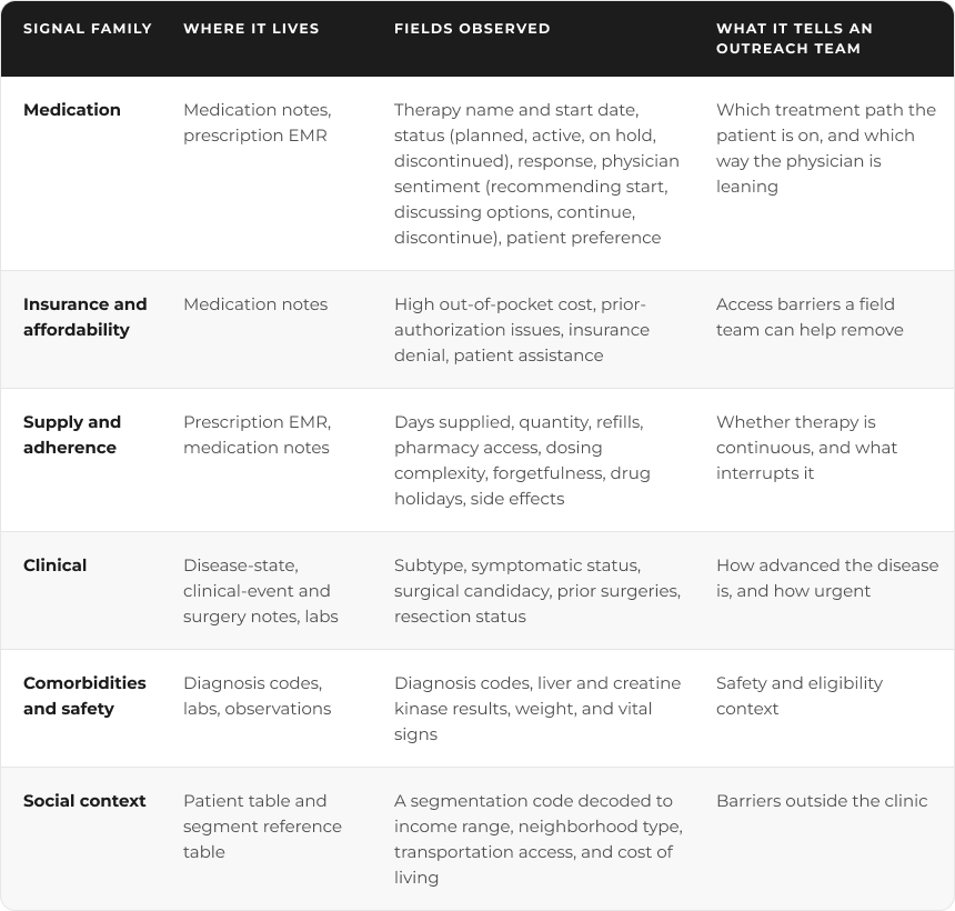
The catch is timing. Only signals documented before the first systemic prescription describe the path to therapy. The same fields after that date, such as response and adverse events, describe the outcome. That is why the rest of this article is about leakage: a signal ranking built on post-therapy notes would simply rediscover that treated patients have been treated.
Two clocks: when it happened and when you could have known.
Every fact in a note sits on two clocks. Clinical time is when the event occurred. Availability time is when the note recording it was written and filed. A feature is safe only if its availability time falls before the moment of prediction. Leakage, in the standard definition, is a model having access at build time to data it would not have at deployment (Ghani, Walsh and Wang, 2020).
For claims, the two clocks sit close together. A pharmacy fill carries a fill date, and a diagnosis row carries a service date. Notes are where they come apart. A framework paper on AI-derived EHR features describes the core problem: a note recorded after treatment can hold pre-treatment history and post-treatment response in the same document (Information Set Emulation, 2026 preprint). Dropping every post-index note throws away useful baseline history. Using the whole note risks leakage. The authors' route out is to split the note conceptually into its before and after parts, then test whether an extracted feature stays stable when the post-treatment sentences are masked.
That masking test is the idea from this literature I find most transferable, and it is cheap to run. I return to it in the playbook below.
What the evidence shows
Note leakage is measurable. A 2026 study of Brazilian ICU notes compared mortality models restricted to the first 24 hours with models given unrestricted notes. Restricted models reached an AUROC of 0.78 to 0.83. With unrestricted notes the figure rose to about 0.95, which the authors read as outcome-related information sitting in late documentation. A regex audit flagged leakage signals in 21.13% of notes, and an LLM-based audit caught further semantic cases that the patterns missed (Alves et al., 2026).
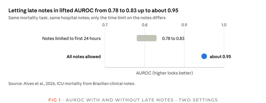
The gap is the cost of a leaked feature: a model that looks about 0.12 to 0.17 AUROC better in development and cannot reproduce that on a patient who has not yet been treated.
Timestamp filtering alone does not close the gap. A 2026 preprint on next-day discharge after elective spine surgery (1,251 patients) points out that documentation often reflects decisions and care plans before they are conducted. Models can then pick up lexical shortcuts that encode future information even when notes are filtered by date. The mitigations it reviews include time-based filtering, excluding discharge summaries and rule-based removal of explicit outcome phrases (arXiv 2602.15852).
The same pattern shows up outside notes, and the size of the effect is instructive. In an audit of clinical-trial outcome prediction, permitting one field that is only known after the fact, actual enrollment, raised ROC-AUC to 0.851. The authors attribute an apparent gain of 0.148 to leakage rather than to better prediction and conclude that the prediction moment should be defined before the predictor is optimized (NeurIPS 2026 audit).
In practice, a leaked feature rarely looks wrong. It looks like a strong result.
What claims work already taught us?
Three lessons from claims-based patient finding carry over to notes.
- Fix the clock per patient, not per calendar.On a rare-disease cohort, my first design used a flat calendar window: take data from a fixed year onward. The client flagged the flaw. For patients who started systemic therapy after that cutoff, the window still captured months of post-initiation data, so the model was learning the consequences of treatment instead of risk factors. The fix was a per-patient landmark. Each patient gets their own start and end date, and every feature function reads from one shared helper that applies a global floor plus the patient window. Changing the time filter now means editing one function.This is the logic of landmark analysis in survival work. Standard Cox regression and Kaplan-Meier methods assume every covariate is known at the start of follow-up, so covariates that arise later need a landmark or time-dependent treatment (Zabor and Assel, 2023). A landmark design defines groups by events that occurred before the landmark and counts outcomes only after it (Gleiss, Oberbauer and Heinze, 2018). Replace "events" with "notes" and the rule is unchanged.
- Do not let reporting lag masquerade as signal.In one comparison, more than 75% of open-claims events were available within three weeks, whereas closed claims took 17 weeks (Weckstein et al.). Recent months are therefore under-counted, and a visit count near the cutoff partly measures how mature the data are. In my experience, binary presence of an event over a long window is more stable than a volume count, so I use it.
- Know what each source can see.An EHR only records care delivered inside its own system. In a study linking claims to two EHR systems, patients in the lowest quartile of EHR continuity had 72-81% of short-term outcome events captured but only 21-31% of long-term ones (Lin et al., 2022). For note features, this means a missing note is not evidence that nothing happened.
A playbook for note-derived features
The routine below is the one I run before a note feature reaches a model. Steps 1 to 3 prevent leakage; steps 4 to 7 detect what slipped through.
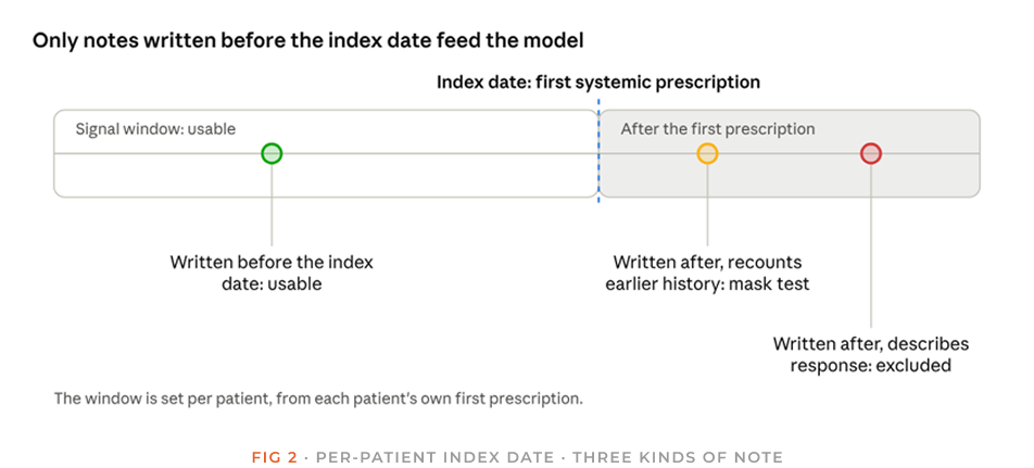
The index date moves from patient to patient, so the picture is drawn once and applied to each patient's own timeline. A note's authoring date, not the date of the visit it describes, decides which side it falls on.
- Define the prediction moment per patient.Set an index date for each patient before writing any feature code. Everything a feature uses must be available on or before it.
- Carry two dates per note.Store the encounter date and the date the note was authored or filed, and filter on the later one. A note about a visit in March that was written in June is a June fact.
- Route every source through one windowing helper.Claims and notes share the same function, a global floor plus a per-patient window, so a rule change cannot be applied to one source and forgotten in another.
- Mask and rerun.For notes written near or after the index date, mask sentences about treatment, response and discharge, rerun the extractor, and drop any feature whose value moves beyond a tolerance you set in advance (Information Set Emulation, 2026 preprint).
- Audit for outcome language.Scan source text for the drug names, start-of-therapy phrases and endpoint wording that define your target. A regex pass catches the obvious cases, and an LLM pass can catch paraphrases (Alves et al., 2026).
- Attack the features with a model.Train a gradient-boosted classifier (I use CatBoost) to predict the outcome flag from the candidate features alone. A feature that carries most of the signal, or a near-perfect score from one feature, is a leakage suspect until proven otherwise. Treat importance rankings as a prompt for review, not a verdict.
- Validate forward in time.Random k-fold shuffles future records into training sets, so hold out later periods instead (Ghani, Walsh, and Wang, 2020).
A worked example
Here is how the routine played out on a rare-disease cohort built from claims and EMR data, with the client, drugs and patient identifiers left out.
The data landscape.
The environment held twenty-three tables and 264 variables, and thirteen of the tables were keyed to a patient. Five of those were NLP-derived concept tables (diagnosis, disease state, medication, surgery, and clinical events). Raw note text sat in a separate table, split into chunks, with up to twelve chunks per note in the sample I profiled. Chunks must be reassembled into the full note before any date window is applied, so a note is kept or dropped as a unit.
Three clocks, not two.
The note tables I worked with carried an encounter identifier, the note's own timestamp and a separate processing date, and the processing date fell into three batches. The encounter, the authoring time and the vendor's load time are different facts. Filtering on the processing date would have been wrong in both directions: it can admit a note written after the index date or hide one written well before it.
The label hides in unexpected tables.
The medication notes were the obvious risk, since they hold therapy status, response and its date, and the physician's stated intent to start or stop. Each of those exists only because therapy happened. The less obvious case was a diagnosis-concept note whose free-text detail field, in a sample I reviewed, stated that the patient was prescribed the therapy. A feature built from that table would have carried the label without anyone intending it. This is the argument for auditing text by content rather than by table name.
Free text finds patients that codes miss.
Of 1,858 patients in a diagnosis-code-defined cohort, 81 (about 4.4%) had either of two approved therapies on record. Of those 81, 38 (about 47%) were identified only through the free-text prescription description, not through the structured drug fields. Positives are scarce, so recovering them matters, but each recovered record needs the same date discipline as the structured ones.
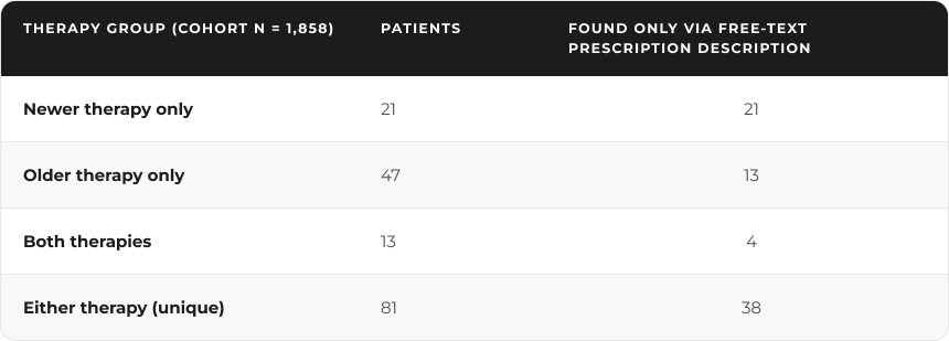
The patients were first found by diagnosis code. The prescription text then supplied their drug exposure, so the structured fields alone would have understated it. In this sample, every patient on the newer therapy alone appears in the free-text-only group, so a structured-field search would have missed that whole group. Setting the signal window to everything before each patient's first prescription gave 31 patients in the newer-therapy group instead of 34, and the overlap fell from 13 to 11. With groups this small, every patient lost for any reason is a visible share of the cohort.
Dates need sanity checks.
Two patients in one therapy cohort showed a first prescription dated before that drug's approval. That can be trial or early-access use, or a date error, and either way it should be resolved before anything is computed relative to that date.
Where LLM extraction fits
Large language models make note extraction easier, and they add a leakage risk of their own: a model that reads a whole note can extract a post-index fact. Two design choices help.
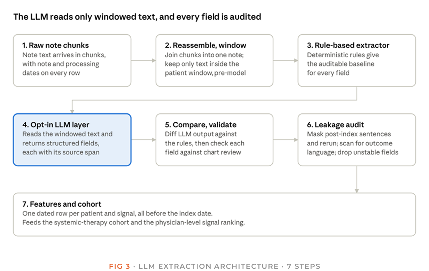
Read it in two passes. The first three boxes prepare and baseline the text, and the date window is applied before the model sees anything. The last four add the LLM, check every field it returns, and only then let a field become a feature.
First, apply the date window to the text before it reaches the model, not to the extracted values afterward. By then the model has already seen what it should not have.
Second, keep the LLM as an opt-in layer on top of a rule-based extractor. The deterministic output stays the auditable baseline, and anything the LLM adds can be compared against it.
Validation should be against manual chart review, field by field, because accuracy varies sharply by field. In one comparison on 182 liver-cancer imaging reports, a general-purpose model reached an overall accuracy of 0.889 against manual review. Across the six extracted data elements it ranged from 0.725 for the sum of tumor diameters to 0.989 for macrovascular invasion. The model ran in an isolated environment approved for protected health information (Ge et al., 2024). A single headline accuracy would have hidden that spread.
What the pre-prescription signals showed
In our data, 91 first-prescription records covered 80 patients, and 70 of the records had at least one note before the first prescription. In those 70, clinical signals are near-universal, and access barriers appear in one record in five.
Cohort ledger.
The diagnosis-code cohort held 1,858 patients, and 81 had a systemic therapy on record. Setting the window before each patient's first prescription left 80 patients and 91 first-prescription records, because 11 patients received both therapies. Of those records, 70 had notes before the first prescription, and every percentage below uses the 70 as its base.
Every flag uses only information dated before that first prescription.
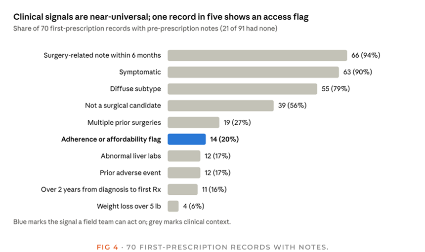
The top bars describe the disease, not the patient's access journey. A "surgery-related note" means a surgical-concept note was written in the six months before the first prescription, usually a discussion of candidacy rather than a procedure. Documented non-candidacy and repeated prior surgery sit in the middle of the chart. Together they describe patients for whom systemic therapy is the live option, which is the pattern a cohort rule should look for.
Missing notes are a signal of their own.
Twenty-one of the 91 records (23%) had no pre-prescription notes at all, 17 on the older therapy and 4 on the newer. Their flags are unknown, not absent. As the claim's lessons showed, a rule that reads "no note" as "no barrier" will understate need (Lin et al., 2022). Treat "no notes" as its own state.
Physician intent is documented for most records with notes.
Among the 42 records with a documented physician stance, 22 were recommending a start, 11 were discussing options, 8 were continuing therapy and 1 was discontinuing. Patient preference was recorded less often, in 26 records, and "willing to try" (9) was the most common answer.
Access barriers are specific.
Fourteen of the 70 records carried an adherence or affordability flag: nine adherence and six affordability, with one record carrying both. Pharmacy access was the most common adherence reason (4 records), and out-of-pocket cost and insurance denial tied on affordability (2 each).
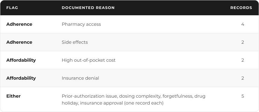
One record lists two reasons, so the reasons total 15 across 14 records. One affordability flag is an insurance approval, which the flag logic counts but a field team would not treat as a barrier. Checking your own flag logic against the raw values is part of the audit.
The mix also shifts with the product but read the next chart with care.
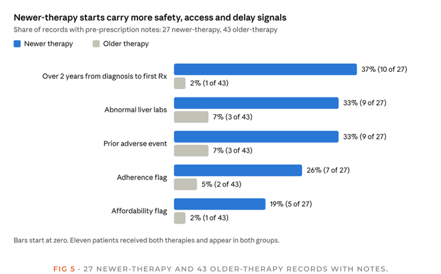
Records for the newer therapy show directionally higher shares of every safety and access signal, and far more long gaps between first diagnosis visit and first prescription. That reflects line of therapy as much as the product: the 11 patients who received both carry their first therapy's history into the second record. With 27 newer-therapy and 43 older-therapy records, one patient moves a bar by two to four points.
These are patient-level shares, not yet physician-level.
The output table I profiled was patient-level and carried no prescriber identifier, so ranking signals by distinct treating physicians, the step the next section describes, needs the provider IDs that sit in the prescription, note, and lab source tables.
From tables to a launch-ready patient and physician list
Every source table did two jobs: it described the patient, and it named the physician behind the record. That is what lets one dataset produce both lists a launch team need, the patients who look like candidates and the physicians and accounts who manage them. Because both come from the same tables, the cohort rule and the physician ranking share one definition of the patient.
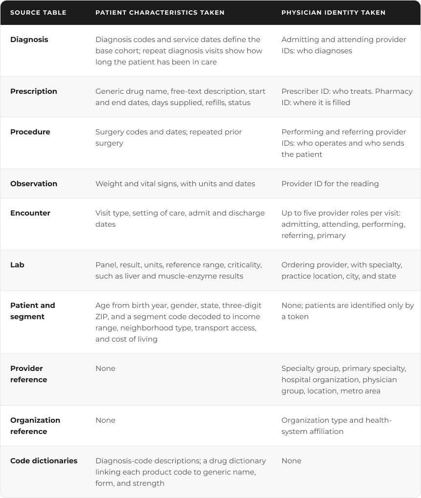
The drug dictionary matters for a second reason. It lets every rule be written by generic name and drug class, so the cohort logic never depends on a brand name and keeps working when a product is added.
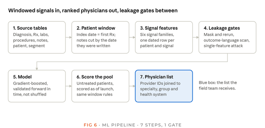
Read it in two rows. The top row turns raw tables into windowed signal features and puts them through the leakage gates. The bottom row trains the model, scores the untreated pool, and converts patient scores into a physician list.
Rule first, model second.
Start with a transparent rule built from the signals many physicians' document. It is easy to explain to a client and easy to check against the 81 treated patients. Then train a gradient-boosted classifier on the same pre-index features to rank the untreated pool and make the rule the baseline it must beat. With positives near 4% of the cohort, judge the model by recall among its top-ranked patients rather than overall accuracy, and use feature attributions to give the field team plain-language reasons for each ranking.
Building the patient profile
- Define the base cohort by diagnosis code. This gave 1,858 patients.
- Mark treatment status from prescriptions. Of the 1,858, 81 had a systemic therapy on record, 38 of them found only through the free-text prescription description. That leaves 1,777 with no systemic therapy on record, the pool the rule scores.
- Cut the history at each treated patient's first prescription. Only information dated before it describes the path to therapy.
- Summarize the path as signals from the six families. In the 70 treated records with pre-prescription notes, 90% were symptomatic, 56% were documented as not surgical candidates, 27% had repeated prior surgery, and 20% carried an adherence or affordability flag. That is the pattern the rule encodes.
- Keep "no notes" as its own state. A patient with no notes is unknown, not clear, so the rule scores that patient on structured fields only and flags the gap.
- Apply the same rule to the untreated pool. Each untreated patient is scored on the same signals, using only information available at the scoring date.
A useful check before launch is a back-test: would the rule have flagged the treated patients before their first prescription? Run on the same patients the rule was built from, the answer is an upper bound. A fair test builds the rule on earlier first prescriptions and scores the later ones.
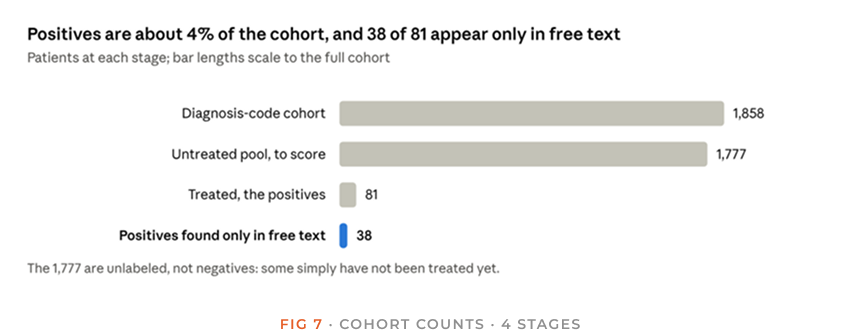
Two modelling consequences follow. With 81 positives, report uncertainty on every metric instead of a single score. And the 1,777 untreated patients are unlabeled rather than negative, so a model trained to separate them from the treated group is partly learning who has not been treated yet, which is exactly the population the launch list is meant to find.
Finding the physicians, with specialty
- Attach each fact to the right physician role. A diagnosis points to the physician who diagnosed, a prescription to the prescriber, a procedure to the surgeon and the referrer, a lab to the ordering provider. These roles need different conversations, so they stay separate.
- Join provider IDs to the provider reference. This adds specialty group, primary specialty, hospital organization, physician group, location, and metro area to every physician.
- Compute per physician. Count the distinct profile-matching patients, the patients already on systemic therapy, and the share of that physician's patients who show each signal. Rank signals by the share of distinct physicians who document them, not by note counts, which reward a few high-volume clinics, and report the physician count beside every percentage.
- Roll up to accounts. Physician group, hospital, and health-system affiliation turn a physician list into an account list, with patient counts per account.
- Segment by role and specialty. Three groups separate naturally: physicians who already prescribe systemic therapy, specialists who diagnose or operate and refer on, and physicians with several matching patients but no systemic prescribing yet. Each needs a different message, and specialty shows which of them can start therapy and which route the patient onward.
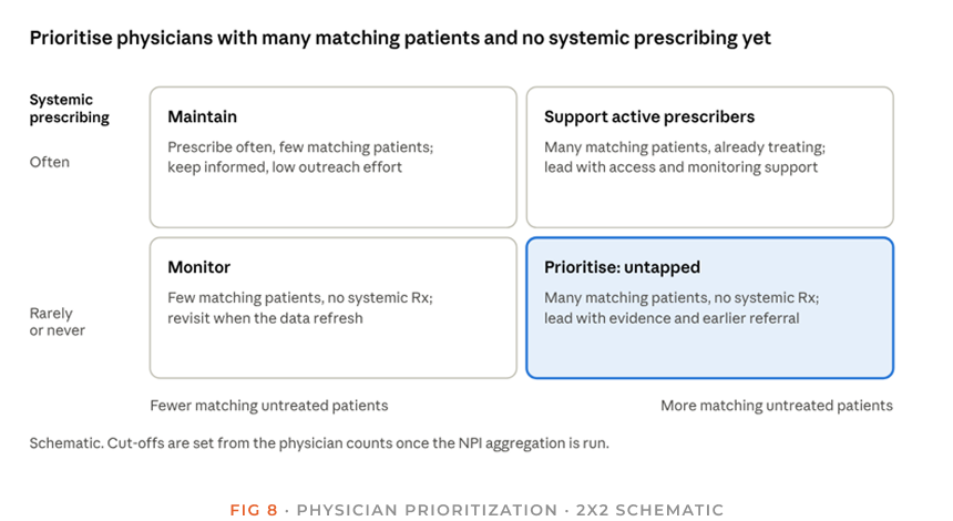
This quadrant is a schematic, not a result. The two axes come straight from the tables: matching untreated patients from the scored pool, and current systemic prescribing from the prescription table by prescriber ID. The shaded quadrant is where outreach changes the most because the patients exist and the physician has not yet had a reason to treat them.
What changes at launch
When a new targeted therapy becomes available, the rule is frozen before launch and rerun on refreshed data at the new scoring date. The output is a ranked list at physician and account level, ordered by the number of matching untreated patients and the signals documented. The signals also choose the message: affordability and adherence flags point to access and support services, liver, and safety flags to monitoring guidance, a documented "discussing options" stance to the clinical evidence, and a long gap from first diagnosis to first prescription to earlier referral.
Three limits apply. The numbers are small, so report the physician count beside every percentage; a signal that most physicians document may rest on a handful. The cohort is a list of candidates, not a treatment recommendation, and the prescribing decision stays with the physician. And because patients are tokenized, the list prioritizes physicians and accounts and is never used to contact or re-identify a patient; the program should go through compliance review before it runs. The evidence in this article is patient-level, and ranking by distinct physicians is the step the provider IDs in the source tables make possible.
 Takeaways
A note is only a feature if it existed, in that form, before the moment you are predicting.
- Give every note two dates, the encounter and the filing, and window on the later one.
- Define the prediction moment per patient and run claims and notes through the same windowing code. On our cohort, windowing per patient shifted group membership: 81 treated patients became 80, and one therapy group fell from 34 to 31, enough to matter at this size.
- Evaluate features adversarial: mask post-index text, audit for outcome language, and try to predict the label from single features.
- Validate forward in time and validate any LLM extractor against chart review field by field. With 81 positives, report uncertainty on every metric and treat untreated patients as unlabeled, not negative.
In my experience, a model built this way scores lower in development than a leaky one. It is also the kind most likely to keep its score once it is asked to find patients who have not been treated yet.
- Alves FAB, Boll HO, Recamonde-Mendoza M. Leakage-Aware Evaluation of Brazilian Clinical Notes for ICU Mortality Prediction: A Study on the BRATECA Dataset. STIL 2026. Link
- Building Safe and Deployable Clinical Natural Language Processing under Temporal Leakage Constraints. arXiv:2602.15852, 2026 preprint. Link
- Information Set Emulation: Causal Certificates for AI Derived EHR Features. arXiv:2609.17777, 2026 preprint. Link
- What Are We Actually Predicting? A Leakage Audit of Clinical Trial Outcome Prediction. NeurIPS 2026. Link
- Ghani R, Walsh J, Wang J. Top 10 ways your machine learning models may have leakage. Data Science for Social Good, 23 January 2020. Link
- Gleiss A, Oberbauer R, Heinze G. An unjustified benefit: immortal time bias in the analysis of time-dependent events. Transplant International 2018; 31:125-130. Link
- Zabor EC, Assel M. On the Need for Landmark Analysis or Time Dependent Covariates. J Urol 2023;209(6):1060-1062. Link
- Weckstein AR, Garry EM, Uppaluri K, et al. Data lag in a large open and closed claims dataset: Navigating the completeness-timeliness tradeoff. HealthVerity poster. Link
- Lin KJ, Jin Y, Gagne J, et al. Longitudinal data discontinuity in electronic health records and consequences for medication effectiveness studies. Clin Pharmacol Ther 2022;111(1):243-251. Link
- Ge J, Li M, Delk MB, Lai JC. A comparison of a large language model vs manual chart review for the extraction of data elements from the electronic health record. Gastroenterology 2024;166(4):707-709. Link

Sourabh Singh Chandel
Data Science Manager
9 years in AI and data science for pharma and healthcare analytics, with earlier work in financial services. Builds real-world evidence, HEOR, patient-finding machine learning and commercial analytics solutions, and leads a growing data science team.
Prepared by PharmSight Research & Analytics for informational purposes only.